DeepSeek-R1 successfully utilizes Group Relative Policy Optimization (GRPO) to improve LLM reasoning capability. This article dives deeper into GRPO, studying its motivation and mechanisms. Also, this article summarizes interesting DeepSeek findings on utilizing RL on LLMs.
In both DeepSeekMath (https://arxiv.org/abs/2402.03300) and DeepSeek-R1 (https://arxiv.org/abs/2501.12948), Group Relative Policy Optimization or GRPO has been utilized to improve LLM reasoning capability in long responses. Especially on math and coding tasks, GRPO has demonstrated convincing performance, enabling DeepSeek models obtain on par performance with GPT-4 and Sonnet-3.5. This article targets a brief analysis over GRPO, and an review on DeepSeek’s findings on utilizing RL.
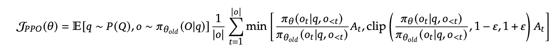
First, let’s brief a short review on PPO. Let $q$ be a query, $P(Q)$ be the query distribution, $\pi_{\text{ref}}$ be a reference model, $o \sim \pi_{\text{ref}}(O\q)$ be a response from the reference model, the PPO objective is defined as
Here, $A_t: O \rightarrow \mathcal{R}$ is the advantage function, which computes the advantage value for each output token $o_t$, which is computed by $V_{\phi} (q, o_{< t}) - r(o_t)$. Here, $V_{\phi}$ is a learned value function, which is usually the same size as $\pi_{\theta}$. So overall, PPO needs at least three models: $\pi_{\theta}$, $\pi_{\text{ref}}$, and $V_{\phi}$, and a potential reward model $r$. This makes PPO occupy much memory space.
The motivation for GRPO is to reduce memory footprint, and it is done via removing the value model $V_{\phi}$. The difference between PPO and GRPO is shown below.
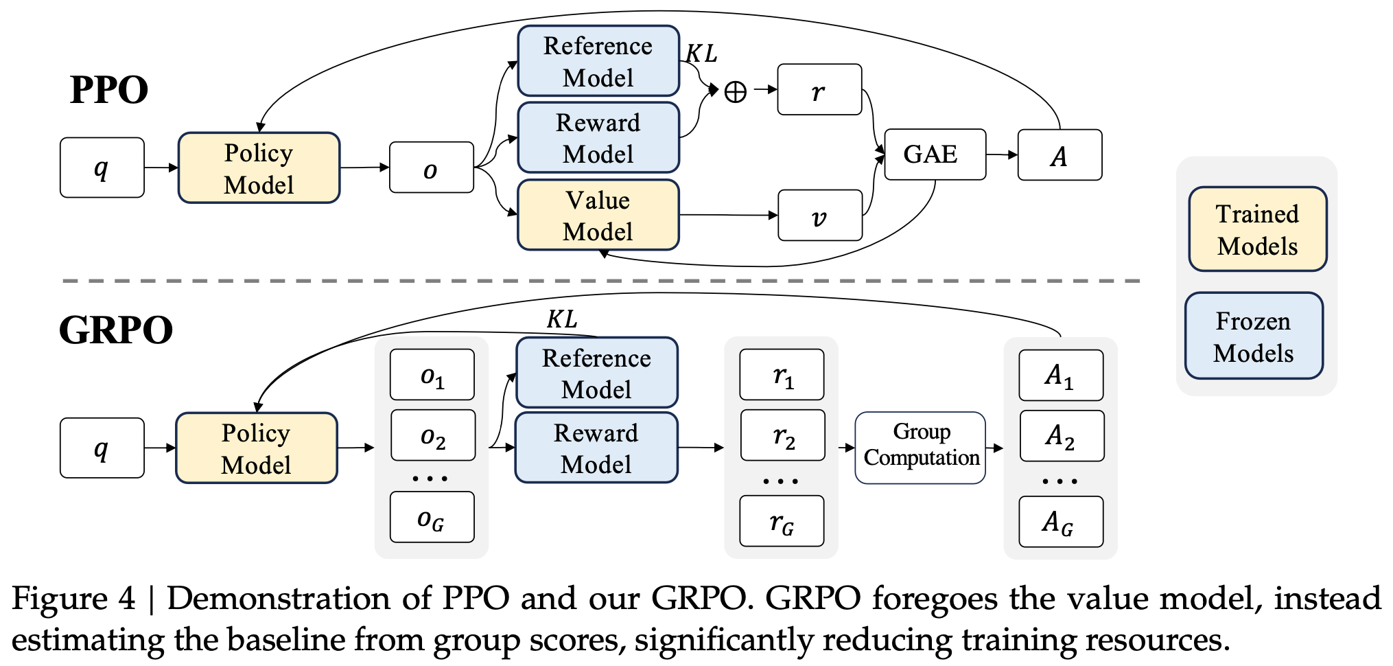
Specifically, instead of using a value function to estimate the value-to-go and compute the advantage, GRPO estimates the value-to-go via taking the mean of rewards across different roll-out trajectories. Let ${o_1, o_2, \ldots, o_G}$ be different roll-out trajectories (responses), $\mathbf{R}={(r_1^{\text{index}(1)}, \ldots, r_1^{\text{index}(K_1)}), \ldots, ((r_G^{\text{index}(1)}, \ldots, r_G^{\text{index}(K_G)}))}$, the value-to-go for $\text{index}_j$ token in the $i$-th trajectory is computed by \(\hat r_i^{\text{index}(j)} = \frac{r_i^{\text{index}(j)} - \text{mean}(\mathbf{R})}{std(\mathbf{R})}\). Then, the advantage value is computed by \(\hat A_{i, t} = \sum_{\text{index}(j) \geq t} r_i^{\text{index}(j)}\).
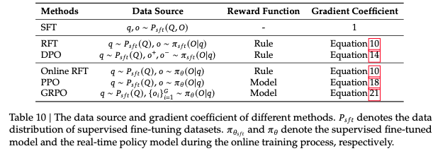
In the DeepSeekMath wort, they consider popular LLM fine-tuning algorithms, including SFT, rejection sampling finetuning (RFT), DPO, online RFT, PPO, and GRPO, and provide a unified formulation on these algorithms:
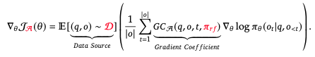
Here, data source $D$ determines the training data (online or offline); reward function $\pi_{rf}$ (ruled-based or model-based); and algorithm $A$ is mostly related to the loss functions, which are responsible to compute the gradient signal basing on the training data and reward signals. Their summarization over popular algorithms is as follows:
Basing on this unified view, different tasks, instruction tuning, distillation, alignment, reasoning, can be viewed as utilizing different RL algorithms to learn from the data.
These are some key takeaways:
Online algorithm significantly outperforms offline (RFT vs Online RFT):
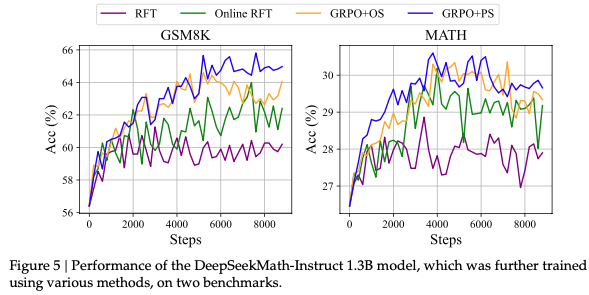
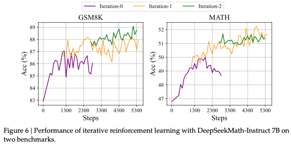
dense reward (step-aware) outperforms sparse reward (GRPO+PS vs GRPO+OS in Figure 5); iterative reward model outperforms fixed reward model (different iterations in Figure 6)